Unit 4 - Video summaries

Video 1

Commodity money is a good that functions as money through exchanges. Representative money is when money is backed up by a metal such as silver or gold. Fiat money is not backed by metal and backed up by the government's word. Money has many functions as well such as being a medium of exchange, store of value, and a unit of account.

Video 2

In mm graphs, Demand slopes downward as it did in the S and D graphs because price and demand have an inverse relationship. Certain factors that can shift the Demand is if there was an incentive to want more money via loans and etc. If people borrowing and spending more money, then the Demand will shift right. In effect it would put upward pressure on the interest rate. If the Fed wants to lower the interest rates in certain times such as an recession, they would increase the money supply.

Video 3

The FED has expansionary and contractionary policies. In expansionary, the reserve requirement (RR) decreases, the discount rate decreases, and the FED buys bonds to expand the money supply. A way to remember this is "buy bonds = big bucks!" In contractionary, the reserve requirement increases, the discount rate increases, and the FED sells bonds to lower the money supply.

Video 4

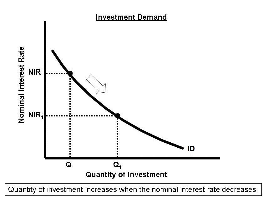
On the loanable funds graph has the same axes as the Money Market graphs. Demand for loadable funds is downward sloping because when interest rates are lower, people demand more money and vice versa. Supply is upward sloping and it also dependent on savings.Savings is a positive factor in this market because the more people save, the more banks will have available. In order to shift the Supply curve left or right there must be an incentive or an lack of a incentive for people to save.  The money market and loanable funds are connected, loanable funds is the source of money for the money market.

Video 5

Banks create money by making loans. The formula for the money multiplier is 1 / reserve requirement. The money multiplier is then multiplied by the amount of money loaned to get the potential total amount of money created in the banking system. This can only be done by assuming that the banks have no excess reserves. If there are excess reserves, then the potential total amount of money is lower.

Video 6

The money market, loanable funds market, and AD/AS market have affects on each other, The money market is where the government gets the money, the demand for loans increase for another source of money(government spending), and the AD increases because government spending is a determinant for the AS/AD market. The equation of exchange is MV=PQ can be used to explain the relationship, as price levels increase the interest rates increase. This can be explained by the "fisher effect." It ultimately means that there is a 1:1 ratio.

Unit 3- Fiscal Policy

Fiscal Policy: Changes in the expenditures or tax revenues of the federal government.

• 2 tools:
• Taxes: The government can increase or decrease taxes.
• Spending: The government can increase or decrease spending.
• 

Deficits, Surpluses, and Debt

• Balanced budget: Revenues = Expenditures
• Budget deficit: Revenues < Expenditures
• Budget surplus: Revenues > Expenditures
• Government debt: Sum of all deficits - sum of all surpluses
• Government must borrow money when it runs a budget deficit.
• Individuals
• Corporations
• Financial institutions
• Foreign entities or foreign governments
• Two options (Fiscal Policy)
• Discretionary Fiscal Policy (action)
• Expansionary (deficit)
• Foreign entities or foreign governments
• Discretionary: Increasing or decreasing government spending in order to return the economy to full employment.
• Automatic: Unemployment compensation and marginal tax rates.
• Takes place without policy makers having to respond to current economic problems.
• Expansionary ("Easy") Fiscal Policy
• Combats a recession
• Increased government spending
• Decreased taxes
• Contractionary ("Tight") Fiscal Policy: 
• Combats inflation
• Decreased government spending
• Increased taxes

Automatic Stabilizers

• Anything that increases the government's budget deficit during a recession and increases its budget surplus during inflation without requiring explicit action by policymakers.
• Transfer payments (Social Security, medicaid/medicare, unemployment, veterans benefits)
• Progressive Tax System
• Average tax rate rises with GDP.
• Proportional
• Average tax rate remains constant as GDP changes.
•   Regressive Tax System
• Average tax rate falls with GDP. 

Unit 3- DI & Multipliers

Disposable Income (DI)

• Income after taxes or net income.
• DI = Gross Income - taxes
• 2 choices for households: consume or save
• Consumption: Household spending
• Amount of DI
• propensity to save
• Do households consume if DI = 0?
• Autonomous consumption
• Dissaving
• Saving: Household NOT spending
• Ability to save constrained by:
• Amount of disposable income
• Propensity to consume
• Do households save if DI = 0?
• NO

APC and APS

• Average Propensity to Consume and Average Propensity to Save
• APC + APS = 1
• 1 - APC = APS
• 1 - APS = APC
• APC > 1: Dissaving
• - APS: Dissaving

MPC and MPS

• Marginal Propensity to Consume (MPC): Fraction of any change in disposable income that is consumed.
• Formula: Change in Consumption / Change in DI
• Marginal Propensity to Save (MPS): Fraction of any change in DI that's saved.
• Formula: Change in savings / Change in DI
• MPC + MPS = 1
• MPC = 1 - MPS
• MPS = 1 - MPC

Spending Multiplier Effect

• An initial change in spending causes a large change in aggregate spending or aggregate demand.
• Multiplier = Change in AD / Change in spending ( C, I, G, or X)
• Calculating Multiplier:
• 1 / 1-MPC or 1 / MPS
• + = increase in spending
• - = decrease in spending
• When the government taxes, the multiplier works in reverse.
• Because money is leaving circular flow.
• Tax multiplier
• -MPC / 1 - MPC
• -MPC / MPS
• If there's a tax cut, multiplier is positive.

Unit 3- Wages

Nominal Wages vs. Real Wages

• Nominal Wages: Amount of money received by a worker per unit of time.
• Real Wages: Amount of goods/services a worker can purchase with their nominal wage. 
• Sticky Wages: Nominal wage level that is set according to an initial price level and does not vary due to labor contracts or other restrictions.

• Recession(Keynesian Range): Fixed price and wages and flexible employment level.
• Output depends upon changes in employment level.
• Intermediate Range; Flexible price and employment level and fixed wages.
• Output depends upon changes in price and employment level.
• Inflationary Range: Flexible price and wages and fixed employment level.
• Output is independent of changes in the price level.
• 

Investment

• Money spent or expenditures on new plants (factories), capital equipment (machinery), technology (hardware and software), new homes, and inventories (goods sold by producers).
• 

Expected Rates of Return

• How does business make investment decisions?
• Cost/Benefit Analysis
• How does business determine benefits?
• Expected rate of return
• How does business count the cost?
• Interest costs
• How does business determine the amount of investment they undertake?
• If expected return > interest cost, then invest.
• If expected return < interest cost, do not invest.

Real (r%) vs. Nominal (i%)

• Nominal is the observable rate of interest.
• Real subtracts out inflation (pi%) and is only know ex post facto.
• How do you compare the real interest rate (r%)/
• r% = i% - pi%
• What then, determines the cost of investment decision? 
• Real interest rate (r%)

Investment Demand Curve (ID)

• What is the shape of the Investment Demand Curve?
• Downward sloping
• Why?
• When interest rates are high, fewer investments are profitable. 
• When interest rates are low, more investments are profitable.
• Cost of production
• Lower costs shift ID > 
• Higher costs shift ID < 
• Business taxes
• Lower business taxes shift ID >
• Higher business taxes shift ID < 
• Technological Change
• New technology shifts ID >
• Lack of technological change shifts ID < 
• Stock of capital
• If an economy is low, then ID >
• If capital increases, then ID < 
• Expectations
• Positive = ID >
• Negative = ID < 

Unit 3 - Aggregate Demand (AD) & Aggregate Supply (AS)

Aggregate Demand Curve

AD = C + I + G + Xn

Shows the demand by consumers, businesses, government, and foreign countries.

Changes in the price level cause a move along the curve.

Why is the AD downward sloping?

1. Real-Balance Effect
• Higher price levels reduce the purchasing power of money.
• This decreases the quantity of expenditures.
• Lower price levels increase purchasing power and expenditures.
2. Interest-Rate Effect
• When the price level increases, lenders need to charge higher interest rates to get a REAL return on their loans.
• Higher interest rates discourage consumer spending and business investment.
3. Foreign Trade Effect
• When U.S. price level rises, foreign buyers purchase fewer U.S. goods and Americans buy more foreign goods.
• Exports fall and imports rise causing real GDP demanded to fall (Xn decreases).

Shifters of Aggregate Demand

• GDP = C + Ig + G + Xn
• Two parts to a shift in AD:
• A change in C, Ig, G, and/or Xn.
• A multiplier effect that produces a greater change than the original change in the 4 components.
• Increase in AD = AD > 
• Decrease in AD = AD < 
• Consumption
• 
• Household spending is affected by:
• Consumer wealth ( ^ wealth, ^ spending)
• Consumer expectations ( ^ expectations, ^ spending)
• Household indebtedness ( if debt decreases, spending ^) 
• Taxes (if taxes decrease, spending ^)

• Gross Private Investment
• Investment spending is sensitive to:
• Real Interest Rate (if interest rate decreases, investment ^)\
• Expected returns ( ^ expected returns = ^ Investment)
• Influenced by: 
• Expectations of future profitability
• Technology
• Degree of excess capacity
• Business taxes
• Government Spending
• ^ government spending = AD > 
• Decrease in government spending = AD < 
• Net Exports
• Sensitive to:
• Exchange rates (International value of $)
• Strong $ = more imports/fewer exports (AD < )
• Weak $ = fewer imports/more exports (AD > )
• Relative Income
• Strong foreign economy = ^ exports (AD >)
• Weak foreign economy = less exports ( AD < )

Aggregate Supply

• Long Run
• Input prices are completely flexible and adjust to changes in the price-level.
• Real GDP is independent of price-level.
• Short Run
• Input prices are sticky and don't adjust to a change in price-level.
• Level of Real GDP is directly related to price level.
• Long Run Aggregate Supply (LRAS)
• Marks the level of full employment in the economy.
• Because input prices are completely flexible in the long-run, changes in price-level do not change firms' real profits.
• LRAS = Vertical
• Changes in SRAS
• Increase in SRAS = >
• Decrease in SRAS = < 
• Per-Unit cost of production =  total input cost / total output

Determinants of SRAS

• Input prices, productivity, and legal institutional environment affect unit cost per production.
• Input prices
• Domestic Resource prices
• Wages (75% of all business costs)
• Cost of capital
• Raw Materials (Commodity prices)
• Foreign Resource prices
• Market power
• Increase in Resource prices = SRAS < 
• Decrease in Resource prices = SRAS >
• Productivity = Total output / total input
• More productivity = lower unit of production = SRAS >
• Less productivity = higher unit of prodution = SRAS <
• Legal Institutional Environment
• Taxes and subsidies
• Government regulation
• Cost of compliance = SRAS <
• Re-regulation = SRAS > 

Full Employment

• FE Equilibrium exists where AD intersects SRAS and LRAS at the same time.
• Recessionary Gap: When equilibrium point occurs below full employment output.
• Inflationary Gap: When equilibrium point occurs beyond full employment output.
• 
• Classical(Vertical) Range: Inflationary 
• Keynesian(Horizontal) Range: Recession